Part 1: Exploring Tensorflow 2 - Keras API
TensorFlow is a free and open-source software library for dataflow and differentiable programming across a range of tasks and it is used for machine learning applications such as neural networks. Tensorflow has grown to become one of the widely adopted ML platforms in the world. TensorFlow offers multiple levels of abstraction so you can choose the right one for your needs. You can build and train models by using the high-level Keras API, which makes getting started with TensorFlow and machine learning easy.
There are a number of good resources to learn Tensorflow, I would mention:
- Hands-On Machine Learning with Scikit-Learn, Keras, and TensorFlow: Concepts, Tools, and Techniques to Build Intelligent Systems 2nd Edition.
It takes you from classical ML to new Tensorflow 2, to broaden your understanding about machine learning in general and more specific about Deep Learning. - Coursera -TensorFlow in Practice Specialization. A Very insightful series, which helps you to discover the tools software developers use to build scalable AI-powered algorithms in TensorFlow.
- Google - Machine Learning Crash Course. A course developed to train internal employees, was updated for the new Tensorflow API.
In this article I’m exploring Sequential and Functional Keras API to create a Deep Neural Network model and use it to predict the likelihood to survive of the Titanic passengers (a well known dataset for data science). I’ll try also to discover best NN parameters for the model using GridSearchCV / RandomizedSearchCV.
My intention is in further blog posts to explore more of the Tensorflow 2 API, like TF.Data for input pipelines, TF.Keras to create CNN (Convolutional Neural Network) and RNN (Recurrent Neural Network) models, deployment strategies and others.
The Notebook is available on Kaggle. Kaggle is the largest data science community where notebooks, datasets are shared and you can even enrol in a ML competition.
Table of Contents:
2. Pre-Processing the data
This is a simplified version of the data pre-processing, checkout the Notebook for detailed flow. Also, it worth to explore the other notebooks for Titanic dataset published by the community.
Pre-processing refers to the transformations applied to our data before feeding it to the algorithm. Data Preprocessing is a technique that is used to convert the raw data into a clean data set.
Deep Learning cannot operate on label data directly. It requires all input variables and output variables to be numeric, threfore the categorical data will be transformed in numbers and numerical values will be scaled for better convergence.
We’ll introduce new features as well, that helps the deep learning algorithms to find better patterns, which will increase prediction accuracy.
import tensorflow as tf
from tensorflow import keras
tf.__version__
'2.1.0'
The data has been split into two groups:
- training set (train.csv) – should be used to build your machine learning models and it has the labels
- test set (test.csv) – should be used to see how well your model performs on unseen data, as I’m using Kaggle the ground truth for each passenger is not provided
# Load dataset
train = pd.read_csv("../input/titanic/train.csv")
test = pd.read_csv("../input/titanic/test.csv")
# Add a column in each dataset before merging
train['Type'] = 'train'
test['Type'] = 'test'
# Merge train and test
data = train.append(test, sort=False)
# Explore the initial data, first 5 rows of the dataset
data.head()
Checkout the original data, before applying feature engineering, encoding and scalling:
2.1. Feature Engineering
Feature engineering is the process of using domain knowledge to extract features from raw data via data mining techniques. These features can be used to improve the performance of machine learning algorithms.
Based on initial exploration of the data, we observed that the Titles from the names (like Miss, Mrs etc) could influence the performance of the model. Therefore we extract those and populate within a new column.
# Extract the Title
for name_string in data['Name']:
    data['Title'] = data['Name'].str.extract('([A-Za-z]+)\.', expand=True)

# Replace the rare titles
mapping = {'Mlle': 'Miss', 'Ms': 'Miss', 'Mme': 'Mrs', 'Major': 'Other',
           'Col': 'Other', 'Dr' : 'Other', 'Rev' : 'Other', 'Capt': 'Other',
           'Jonkheer': 'Royal', 'Sir': 'Royal', 'Lady': 'Royal',
           'Don': 'Royal', 'Countess': 'Royal', 'Dona': 'Royal'}
data.replace({'Title': mapping}, inplace=True)

#Consolidate Parch and SibSp within a single column, named Family_Size.
data['Family_Size'] = (data['Parch'] + data['SibSp']).astype(int)
2.2. Fill in the missing data
Although it is possible to train algorithms with missing values, it’s highly recommended to clean the data.
Strategies to clean up dataset:
- Drop the missing values: Drop the row if a particular feature is missing
- Replace the missing values with mean/median imputation: Calculate the mean or median of the feature and replace it with the missing values. This is an approximation which can add variance to the data set. But the loss of the data can be negated by this method which yields better results compared to removal of rows and columns
# Age is filled with the mean for the corresponding category
data['Age'].fillna(data.groupby(["Sex", "Pclass"])['Age'].transform("mean"), inplace=True)

#Manually add the two missing values for Embarked
data.loc[61,'Embarked'] = 'S'
data.loc[829,'Embarked'] = 'S'

# Fare is filled with the mean.
data['Fare'].fillna(data['Fare'].mean(), inplace = True)
2.3. Encode Categorical and Scale Continuous variables
There are two types of data:
- Categorical : Features whose values are taken from a defined set of values. For instance, days in a week : {Monday, Tuesday, Wednesday, Thursday, Friday, Saturday, Sunday} is a category because its value is always taken from this set. Another example could be the Boolean set : {True, False}
- Numerical : Features whose values are continuous or integer-valued. They are represented by numbers and possess most of the properties of numbers. For instance, number of steps you walk in a day, or the speed at which you are driving your car at.
Encode Categorical Variables
We need to convert all categorical variables into numeric format. The categorical variables we will be keeping are Embarked, Sex and Title.
Scale Continuous variables
Standardization is a useful technique to transform attributes with a Gaussian distribution and differing means and standard deviations to a standard Gaussian distribution with a mean of 0 and a standard deviation of 1.
We can standardize data using scikit-learn with the StandardScaler class.
# Drop the variables that won't be used in the model
data.drop(['Cabin', 'Name', 'Ticket', 'PassengerId', 'SibSp', 'Parch'], axis=1, inplace=True)

# Convert to cateogry dtype
data['Sex'] = data['Sex'].astype('category')
# Convert to category codes
data['Sex'] = data['Sex'].cat.codes

# Encode the categorical values
categorical = ['Embarked', 'Title', 'Pclass']
for cat in categorical:
    data = pd.concat([data,
                    pd.get_dummies(data[cat], prefix=cat)], axis=1)
    del data[cat]

# Scale the numerical values
continuous = ['Age', 'Fare', 'Family_Size']
scaler = StandardScaler()
for val in continuous:
    data[val] = data[val].astype('float64')
    data[val] = scaler.fit_transform(data[val].values.reshape(-1, 1))

# Checkout the data after all transformations have been applied
data.head()
# Split the train and test dataset
train = data[data['Type'] == 'train'].drop(columns = ['Type', 'Survived'])
train_ = data[data['Type'] == 'train']['Survived']
X_train = train.values
y_train = train_.values

test = data[data['Type'] == 'test'].drop(columns = ['Type', 'Survived'])
X_test = test.values
X_test = X_test.astype(np.float64, copy=False)

#Checkout the shape of the training dataset
train.shape
(891, 16)
3. Create the Model.
3.1. TensorFlow 2 & Keras
TensorFlow has been upgraded recently to 2.x version, most notable additions in TensorFlow 2.x comparing with 1.x:
- tf.keras - default TensorFlow’s high-level API for building and training deep learning models.
- Eager execution - is an imperative programming environment that evaluates operations immediately, without building graphs: operations return concrete values instead of constructing a computational graph to run later.
- Distribution Strategy API - makes it easy to distribute and train models on different hardware configurations without changing the model definition.
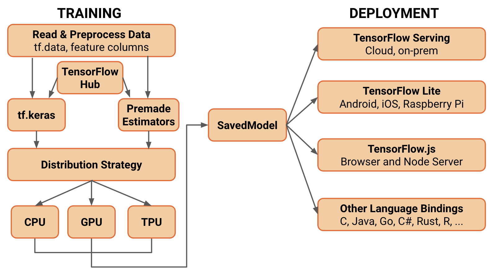
- Standardized SavedModel file format - allows you to run your models with TensorFlow, deploy them with TensorFlow Serving, use them on mobile and embedded systems with TensorFlow Lite, and train and run in the browser or Node.js with TensorFlow.js.
This is just a small subset of features, checkout the official documentation for the latest details. Keep in mind that the framework is growing very rapidly, so there are a number of new additions in the last 2.x APIs.
Keras is a user-friendly API standard for machine learning and it is the central high-level API used to build and train models in TensorFlow 2.x. Importantly, Keras provides several model-building APIs (Sequential, Functional, and Subclassing), so you can choose the right level of abstraction for your project.
The new architecture of TensorFlow 2.x using a simplified, conceptual diagram:
3.2. Keras building blocks
Keras models are made by connecting configurable building blocks together.
In Keras, you assemble layers to build models. A model is a graph of layers. The most common type of model is a stack of layers: the tf.keras.Sequential model.
3.3. TF Keras model using Sequential API
3.3.1. Model architecture
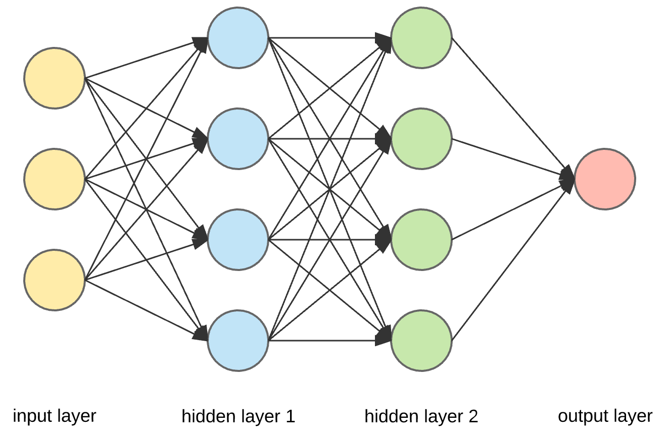
Dense layers are the most basic neural network architecture. In this layer, all the inputs and outputs are connected to all the neurons in each layer.
This is one Neuron computation:
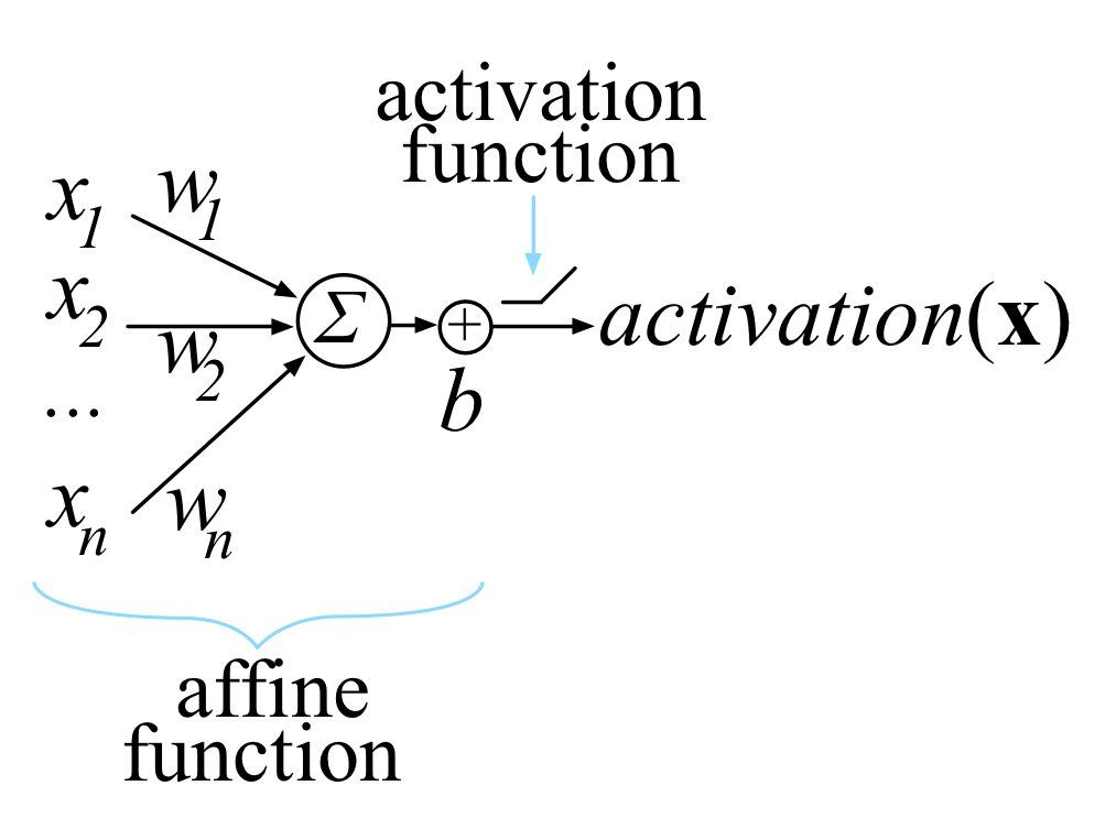
A neural network without an activation function is essentially just a linear regression model. The activation function does the non-linear transformation to the input making it capable to learn and perform more complex tasks. Most known activation functions are: Sigmoid , Tanh and Relu.
It is out of the scope of this article to present the math behind the DNN, but the scope of the training process is to find the best weights that will minimize the cost function, in order to make better predictions.
The simplified process:
- Forward Propagation – given the inputs from previous layer or the input layer, each unit computes the affine function and then apply the activation function. All computed variables on each layers are stored and used by back-propagation.
- Calculate loss function which compare the final output of the model with the actual target in the training data.
- Back-propagation, it goes backwards from right to left, and propagates the error to every node, then calculate each weight’s contribution to the error, and adjust the weights accordingly using gradient descent.
TF Keras Dense Layer implements the operation: output = activation(dot(input, kernel) + bias) where:
- activation is the element-wise activation function passed as the activation argument.
- kernel is a weights matrix created by the layer.
- bias is a bias vector created by the layer.
Now, let’s create a simple model using TF Keras. Sequential model is the simplest kind of Keras model for neural networks that are just composed of a single stack of layers connected sequentially.
# Simple model
model1 = keras.models.Sequential()
# 18 units is dimensionality of the output space.
# input_dim specify the size of the input
model1.add(keras.layers.Dense(18, input_dim = X_train.shape[1], activation = keras.activations.relu))
model1.add(keras.layers.Dense(8, activation = keras.activations.relu))
model1.add(keras.layers.Dense(1, activation = keras.activations.sigmoid))

# Visualize the model
model1.summary()
Model: "sequential"
_________________________________________________________________
Layer (type)                 Output Shape              Param #
=================================================================
dense (Dense)                (None, 18)                306
_________________________________________________________________
dense_1 (Dense)              (None, 8)                 152
_________________________________________________________________
dense_2 (Dense)              (None, 1)                 9
=================================================================
Total params: 467
Trainable params: 467
Non-trainable params: 0
_________________________________________________________________
# further explore the model
weights, biases = model1.layers[1].get_weights()
weights.shape
(18, 8)
3.3.2. Compile the model
tf.keras.Model.compile takes three important arguments:
- optimizer: This object specifies the training procedure. Pass it optimizer instances from the tf.keras.optimizers module, such as tf.keras.optimizers.Adam or tf.keras.optimizers.SGD. If you just want to use the default parameters, you can also specify optimizers via strings, such as ‘adam’ or ‘sgd’.
- loss: The function to minimize during optimization. Common choices include mean square error (mse), categorical_crossentropy, and binary_crossentropy. Loss functions are specified by name or by passing a callable object from the tf.keras.losses module.
- metrics: Used to monitor training. These are string names or callables from the tf.keras.metrics module.
- Additionally, to make sure the model trains and evaluates eagerly, you can make sure to pass run_eagerly=True as a parameter to compile.
# Compiling our model
model1.compile(optimizer = keras.optimizers.SGD(),
               loss = keras.losses.binary_crossentropy,
               metrics = [tf.keras.metrics.binary_accuracy])
This is equivalent to:
model1.compile(loss=“binary_crossentropy”, optimizer=“sgd”, metrics=[“accuracy”])
3.3.3. Train the model
tf.keras.Model.fit takes three important arguments:
- epochs: Training is structured into epochs. An epoch is one iteration over the entire input data (this is done in smaller batches).
- batch_size: When passed NumPy data, the model slices the data into smaller batches and iterates over these batches during training. This integer specifies the size of each batch. Be aware that the last batch may be smaller if the total number of samples is not divisible by the batch size.
- validation_data: When prototyping a model, you want to easily monitor its performance on some validation data. Passing this argument—a tuple of inputs and labels—allows the model to display the loss and metrics in inference mode for the passed data, at the end of each epoch.
- validation_split: Float between 0 and 1. Same as validation_data, but the but it use a fraction of the training data to be used as validation data. The model will set apart this fraction of the training data, will not train on it, and will evaluate the loss and any model metrics on this data at the end of each epoch.
history = model1.fit(X_train, y_train, epochs=100, validation_split=0.2)

val_acc = np.mean(history.history['val_binary_accuracy'])
print("\n%s: %.2f%%" % ('val_acc', val_acc*100))
val_acc: 80.47%
history.params
{'batch_size': 32,
 'epochs': 100,
 'steps': 23,
 'samples': 712,
 'verbose': 0,
 'do_validation': True,
 'metrics': ['loss', 'binary_accuracy', 'val_loss', 'val_binary_accuracy']}
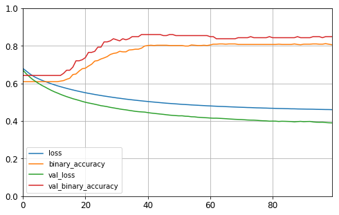
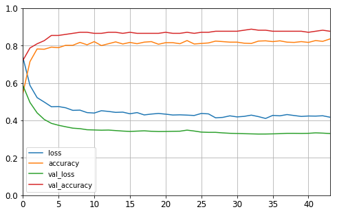
# Plot the learning curves
pd.DataFrame(history.history).plot(figsize=(8, 5))
plt.grid(True)
plt.gca().set_ylim(0, 1)
plt.show()
3.3.4 Predict on the Test data and submit to Kaggle
If you participate in a Kaggle competion, you may want to submit the model predictions and receive the calculated score from Kaggle. This way you can verify if the model generalize well or not.
# Calculate predictions, this model scores 0.76555 on Kaggle

submission = pd.read_csv("../input/titanic/gender_submission.csv", index_col='PassengerId')
submission['Survived'] = model1.predict(X_test)
submission['Survived'] = submission['Survived'].apply(lambda x: round(x,0)).astype('int')
submission.to_csv('Titanic_model1.csv')
3.4. Keras Model using Functional API
Although it is possible to use Keras Sequential API, for next model as the layers are added one after another, for the sake of this exercise I’ll create the model using Functional API.
The Keras functional API is the way to go for defining complex models, such as multi-output models, directed acyclic graphs, or models with shared layers.
Comparing with previuos model:
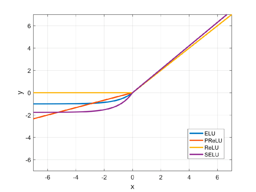
- Elu is used as an activation function, it looks a lot like the ReLU function but it has a nonzero gradient for z < 0
- I’m using Dropout, which is one popular technique for regularization, however L1, L2 and Max-Norm can be used as well.
# Create the model, the input for each layer is manually passed
input_ = keras.layers.Input(shape=X_train.shape[1:])
hidden1 = keras.layers.Dense(36, activation="elu")(input_)
drop1 = keras.layers.Dropout(rate=0.2)(hidden1)
hidden2 = keras.layers.Dense(18, activation="elu")(drop1)
drop2 = keras.layers.Dropout(rate=0.2)(hidden2)
hidden3 = keras.layers.Dense(8, activation="elu")(drop2)
output = keras.layers.Dense(1, activation="sigmoid")(hidden3)
model2 = keras.models.Model(inputs=[input_], outputs=[output])

# Print the model
model2.summary()
Model: "model"
_________________________________________________________________
Layer (type)                 Output Shape              Param #
=================================================================
input_1 (InputLayer)         [(None, 16)]              0
_________________________________________________________________
dense_3 (Dense)              (None, 36)                612
_________________________________________________________________
dropout (Dropout)            (None, 36)                0
_________________________________________________________________
dense_4 (Dense)              (None, 18)                666
_________________________________________________________________
dropout_1 (Dropout)          (None, 18)                0
_________________________________________________________________
dense_5 (Dense)              (None, 8)                 152
_________________________________________________________________
dense_6 (Dense)              (None, 1)                 9
=================================================================
Total params: 1,439
Trainable params: 1,439
Non-trainable params: 0
_________________________________________________________________
# Compile the model
model2.compile(optimizer = 'nadam',
               loss = 'binary_crossentropy',
               metrics = ['accuracy'])
The fit() method accepts a callbacks argument that lets you specify a list of objects that Keras will call at the start and end of training, at the start and end of each epoch, and even before and after processing each batch.
tf.keras.callbacks.EarlyStopping is usefull when you want to stop training when a monitored quantity has stopped improving. The number of epochs can be set to a large value since training will stop automatically when there is no more progress.
# configure EarlyStopping and ask to restore the best weights
early_stopping_cb = keras.callbacks.EarlyStopping(patience=10, restore_best_weights=True)
Train the model with callbacks:
history2 = model2.fit(X_train, y_train, epochs=100, validation_split=0.2, callbacks=[early_stopping_cb])

# Calculate  validation accuracy
val_acc = np.mean(history2.history['val_accuracy'])
print("\n%s: %.2f%%" % ('val_acc', val_acc*100))
val_acc: 86.41%
# Plot the learning curves
pd.DataFrame(history2.history).plot(figsize=(8, 5))
plt.grid(True)
plt.gca().set_ylim(0, 1)
plt.show()
# Calculate predictions, this model scores 0.77511 on Kaggle
submission2 = pd.read_csv("../input/titanic/gender_submission.csv", index_col='PassengerId')
submission2['Survived'] = model2.predict(X_test)
submission2['Survived'] = submission['Survived'].apply(lambda x: round(x,0)).astype('int')
submission2.to_csv('Titanic_model2.csv')
3.5. Hyperparameter Tuning
Create the model, in such way to be configurable. The dynamic model allows you to try and find out the best model hyperparameters.
def build_model(input_shape=[16], n_hidden=1, n_neurons=30, activation = 'relu', optimizer = 'SGD'):
    model = keras.models.Sequential()
    model.add(keras.layers.InputLayer(input_shape=input_shape))
    i = 1
    for layer in range(n_hidden):
        model.add(keras.layers.Dense(n_neurons/i, activation=activation))
        if n_neurons > 20:
            model.add(keras.layers.Dropout(rate=0.2))
            i = i + 2
    model.add(keras.layers.Dense(1, activation='sigmoid'))
    model.compile(loss="binary_crossentropy", optimizer=optimizer, metrics=['accuracy'])
    return model
In Keras there is a wrapper for using the Scikit-Learn API with Keras models, that has 2 classes:
- KerasClassifier: Implementation of the scikit-learn classifier API for Keras.
- KerasRegressor: Implementation of the scikit-learn regressor API for Keras.
KerasClassifier object is a thin wrapper around the Keras model built using build_model(). The object can be used like a regular Scikit-Learn regressor so we can train, evaluate and make predictions using it.
model3 = keras.wrappers.scikit_learn.KerasClassifier(build_fn=build_model)
history3 = model3.fit(X_train, y_train, epochs=100,
              validation_split=0.2,
              callbacks=[keras.callbacks.EarlyStopping(patience=10)])
val_acc = np.mean(history3.history['val_accuracy'])
print("\n%s: %.2f%%" % ('val_acc', val_acc*100))
val_acc: 82.82%
Random search for hyper parameters.
In contrast to GridSearchCV, not all parameter values are tried out, but rather a fixed number of parameter settings is sampled from the specified distributions. The number of parameter settings that are tried is given by n_iter.
Activation functions:
- Relu - Applies the rectified linear unit activation function: max(x, 0)
- Selu - Scaled Exponential Linear Unit (SELU): scale * x if x > 0 and scale * alpha * (exp(x) - 1) if x < 0
- Elu - Exponential linear unit: x if x > 0 and alpha * (exp(x)-1) if x < 0
Optimizers:
- SGD - stochastic gradient descent, is the “classical” optimization algorithm. In SGD the gradient is computed for the network loss function with respect to each individual weight in the network. Each forward pass through the network results in a certain parameterized loss function, and use the calculated gradients with the learning rate to move the weights in whatever direction its gradient is pointing.
- Adagrad - scales down the gradient vector along the steepest dimensions
- RMSprop - accumulate only the gradients from the most recent iterations (as opposed to all the gradients since the beginning of training)
- Adam - stands for adaptive moment estimation, combines the ideas of momentum optimization and RMSProp
from sklearn.model_selection import RandomizedSearchCV

param_distribs = {
    "n_hidden": [1, 2, 3, 4],
    "n_neurons": [6, 18, 30, 42, 56, 77, 84, 100],
    "activation": ['relu', 'selu', 'elu'],
    "optimizer": ['SGD', 'RMSprop', 'Adam'],
}

rnd_search_cv = RandomizedSearchCV(model3, param_distribs, n_iter=10, cv=3, verbose=2)
rnd_search_cv.fit(X_train, y_train, epochs=100, validation_split=0.2)

# Print the best found hyperameters
rnd_search_cv.best_params_
{'optimizer': 'Adam', 'n_neurons': 42, 'n_hidden': 4, 'activation': 'selu'}
It didn’t work out for me, as each time I run it I got different results, but I guess it worth to know that it is posible to use these valuable Scikit Learn libraries with Keras:
{‘optimizer’: ‘RMSprop’, ’n_neurons’: 84, ’n_hidden’: 3, ‘activation’: ‘selu’}
{‘optimizer’: ‘Adam’, ’n_neurons’: 77, ’n_hidden’: 4, ‘activation’: ’elu’}
{‘optimizer’: ‘RMSprop’, ’n_neurons’: 30, ’n_hidden’: 1, ‘activation’: ‘relu’}
{‘optimizer’: ‘RMSprop’, ’n_neurons’: 6, ’n_hidden’: 4, ‘activation’: ‘selu’}
{‘optimizer’: ‘SGD’, ’n_neurons’: 100, ’n_hidden’: 4, ‘activation’: ’elu’}
Assume that you’ve found better hyperparameters, it can be easily apply to your model.
model4 = build_model(n_hidden=4, n_neurons=77, input_shape=[16], activation = 'elu', optimizer = 'Adam')

print(model4.summary())
Model: "sequential_33"
_________________________________________________________________
Layer (type)                 Output Shape              Param #
=================================================================
dense_116 (Dense)            (None, 77)                1309
_________________________________________________________________
dropout_67 (Dropout)         (None, 77)                0
_________________________________________________________________
dense_117 (Dense)            (None, 25)                1950
_________________________________________________________________
dropout_68 (Dropout)         (None, 25)                0
_________________________________________________________________
dense_118 (Dense)            (None, 15)                390
_________________________________________________________________
dropout_69 (Dropout)         (None, 15)                0
_________________________________________________________________
dense_119 (Dense)            (None, 11)                176
_________________________________________________________________
dropout_70 (Dropout)         (None, 11)                0
_________________________________________________________________
dense_120 (Dense)            (None, 1)                 12
=================================================================
Total params: 3,837
Trainable params: 3,837
Non-trainable params: 0
_________________________________________________________________
None
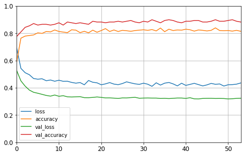
history4 = model4.fit(X_train, y_train, epochs=100,
                     validation_split=0.2, callbacks=[early_stopping_cb])

# Plot the learning curves, no much improvements as you can see
pd.DataFrame(history4.history).plot(figsize=(8, 5))
plt.grid(True)
plt.gca().set_ylim(0, 1)
plt.show()
Using deep learning for this dataset may be overkill, as this dataset is tiny, however it was fun to play with Tensorflow 2.x and Keras API. The performance was not the primary goal of this article, but if you are looking for best performance, maybe using Ensembling/Stacking with RandomForest and GradientBoosting could work better for this dataset.
Anyway, I hope you enjoyed the rundown.